Basics
Welcome! This tutorial will guide you though the main functions in asilib.
First off, we need to import the necessary packages.
[1]:
from datetime import datetime, timedelta
from IPython.display import Video
import numpy as np

import matplotlib.pyplot as plt
import matplotlib.colors
import asilib
import asilib.asi
import asilib.map

plt.style.use('dark_background')

print(f'asilib version: {asilib.__version__}')
asilib version: 0.30.1
First of all, you should know where the data and movies are saved to. This information is in asilib.config and can be changed with python3 -m asilib config to configure asilib.
[2]:
asilib.config
[2]:
{'ASILIB_DIR': PosixPath('/home/msshumko/research/asilib/asilib'),
 'ASI_DATA_DIR': PosixPath('/mnt/f/asilib-data'),
 'ACKNOWLEDGED_ASIS': []}
As you can guess, asilib.config['ASILIB_DIR'] is the directory where this code resides, asilib.config['ASI_DATA_DIR'] is the directory where the data is saved to.
Plot a single image
The core of asilib is the asilib.Imager class. It provides an intuitive interface to load, plot, animate, and analyze auroral images. Normally, you do not need to call asilib.Imager() directly. Instead, you initialize an asilib.Imager object via a ASI interface function, such as asilib.asi.themis, asilib.asi.rego, or asilib.asi.trex_nir. Let’s see how this works by plotting a fisheye lens image from a THEMIS imager at Athabasca (ATHA). We will show the aurora studied in:
Liu, J., Lyons, L. R., Archer, W. E., Gallardo-Lacourt, B., Nishimura, Y., Zou, Y., … Weygand, J. M. (2018). Flow shears at the poleward boundary of omega bands observed during conjunctions of Swarm and THEMIS ASI. Geophysical Research Letters, 45, 1218– 1227. https://doi.org/10.1002/2017GL076485
[3]:
location_code = 'ATHA'
time = datetime(2008, 3, 9, 9, 18, 0)  # You can supply a datetime object or a ISO-formatted time string.

asi = asilib.asi.themis(location_code, time=time)
ax, im = asi.plot_fisheye(cardinal_directions='news')
plt.colorbar(im)
ax.axis('off');

That is it! By calling the asilib.asi.themis() function, we create an asilib.Imager() object—with uniform interface. In other words, plotting a fisheye image (Imager.plot_fisheye()) is the same for THEMIS, REGO, TREx, or any other ASI supported by asilib. This is what makes asilib so powerful.
It is also easy to map the ASI fisheye lens image to a geographic map using the Imager.plot_map() method. In the code box below, the first line creates a geographic map centered on Athabasca and the second line projects the image onto the map.
Note 1: If latitude or longitude bounds are not provided, Imager.plot_map() defaults to a map of North America. Note 2: We derived the lon_bounds and lat_bounds using the Imager.skymap dictionary which we describe in more detail below.
[6]:
lon_bounds = (np.nanmin(asi.skymap['lon']), np.nanmax(asi.skymap['lon']))
lat_bounds = (np.nanmin(asi.skymap['lat']), np.nanmax(asi.skymap['lat']))
ax = asilib.map.create_simple_map(lon_bounds=lon_bounds, lat_bounds=lat_bounds)
asi.plot_map(ax=ax);

Notice that you did not need to explicitly download or load the data. The ASI Interface Function downloads the necessary image and skymap files, while asilib.Imager() loads data as needed, also known as the “lazy” mode. This preserves your computer’s memory at the expense of processing speed. Alternatively, you can load all of the data into memory at once with the “eager” mode.
[5]:
asi_data = asi.data
[6]:
asi_data.time
[6]:
datetime.datetime(2008, 3, 9, 9, 18, 0, 50605)
[7]:
asi_data.image.shape
[7]:
(256, 256)
[8]:
asi_data.image
[8]:
array([[2536, 2616, 2554, ..., 2572, 2537, 2546],
       [2582, 2582, 2620, ..., 2562, 2613, 2608],
       [2544, 2560, 2568, ..., 2588, 2526, 2550],
       ...,
       [2525, 2546, 2553, ..., 2612, 2541, 2629],
       [2545, 2596, 2698, ..., 2510, 2568, 2569],
       [2502, 2577, 2602, ..., 2514, 2617, 2576]],
      shape=(256, 256), dtype=uint16)
Data availability
How would someone look-up if there is ASI data available? For this we can use the asilib.asi.themis_available() and asilib.asi.plot_themis_available() functions to tell us if each ASI was on in each hour
[9]:
themis_available = asilib.asi.themis_available(time_range=(datetime(2008, 3, 9, 0, 0, 0), datetime(2008, 3, 10, 0, 0, 0)))
themis_available.head()
Checking THEMIS ASI availability: |#####################################| 100%
[9]:
| location_code | ATHA | CHBG | EKAT | FSIM | FSMI | FYKN | GAKO | GBAY | GILL | INUV | ... | NRSQ | PGEO | RANK | SNAP | SNKQ | TALO | TPAS | WHIT | YKNF | PINA |
|---|---|---|---|---|---|---|---|---|---|---|---|---|---|---|---|---|---|---|---|---|---|
| 2008-03-09 00:00:00 | False | True | False | False | False | False | False | True | False | False | ... | False | False | False | False | True | False | False | False | False | False |
| 2008-03-09 01:00:00 | False | True | False | False | False | False | False | True | True | False | ... | False | False | True | False | True | False | True | False | False | True |
| 2008-03-09 02:00:00 | True | True | False | False | True | False | False | True | True | False | ... | False | False | True | False | True | False | True | False | True | True |
| 2008-03-09 03:00:00 | True | True | False | True | True | False | False | True | True | False | ... | False | True | True | False | True | False | True | False | True | True |
| 2008-03-09 04:00:00 | True | True | False | True | True | True | True | True | True | True | ... | False | True | True | False | True | False | True | True | True | True |
5 rows × 24 columns
[20]:
themis_available, ax = asilib.asi.plot_themis_available(
    time_range=(datetime(2008, 3, 9, 0, 0, 0), datetime(2008, 3, 10, 0, 0, 0))
    )
Checking THEMIS ASI availability: |#####################################| 100%

Lastly, here is how you can determine which ASIs took data on this night. Here we use the pd.DataFrame.any() method as none of the THEMIS ASIs were on for the full time period. Use pd.DataFrame.all() if you have a shorter time period and want to make sure that all imagers were on the whole time.
[27]:
themis_available.any()
[27]:
location_code
ATHA     True
CHBG     True
EKAT    False
FSIM     True
FSMI     True
FYKN     True
GAKO     True
GBAY     True
GILL     True
INUV     True
KAPU     True
KIAN     True
KUUJ     True
MCGR     True
NRSQ    False
PGEO     True
RANK     True
SNAP    False
SNKQ     True
TALO    False
TPAS     True
WHIT     True
YKNF     True
PINA     True
dtype: bool
[32]:
themis_available.columns[themis_available.any()]
[32]:
Index(['ATHA', 'CHBG', 'FSIM', 'FSMI', 'FYKN', 'GAKO', 'GBAY', 'GILL', 'INUV',
       'KAPU', 'KIAN', 'KUUJ', 'MCGR', 'PGEO', 'RANK', 'SNKQ', 'TPAS', 'WHIT',
       'YKNF', 'PINA'],
      dtype='str', name='location_code')
And we can also determine which ASIs took data right at 2008-03-09T09:18:00
[33]:
themis_available = asilib.asi.themis_available(time='2008-03-09T09:18:00')
[42]:
themis_available[themis_available].index
[42]:
Index(['ATHA', 'CHBG', 'FSIM', 'FSMI', 'FYKN', 'GAKO', 'GBAY', 'GILL', 'INUV',
       'KAPU', 'KIAN', 'KUUJ', 'MCGR', 'PGEO', 'RANK', 'SNKQ', 'TPAS', 'WHIT',
       'YKNF', 'PINA'],
      dtype='str', name='location_code')
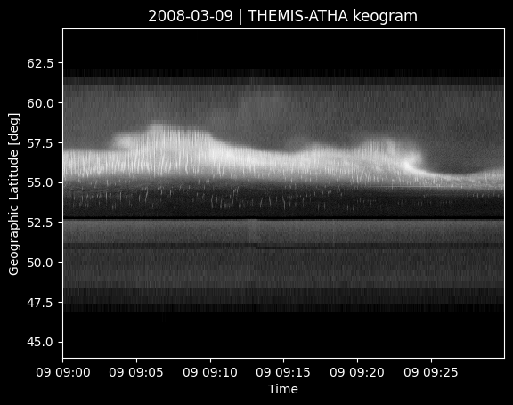
Plot a Keogram
Imager.plot_keogram() plots a keogram through the meridian. Alternatively, you can specify a custom path using (latitude, longitude coordinates).
By default, the y-axis is geographic latitude. If you set aacgm=True, the keogram’s vertical axis will be magnetic latitude estimated using the aacgmv2 Python package. It implements the Altitude-adjusted corrected geomagnetic coordinates defined in Shepherd 2014.
[8]:
time_range = [datetime(2008, 3, 9, 9, 0, 0), datetime(2008, 3, 9, 9, 30, 0)]
asi2 = asilib.asi.themis(location_code, time_range=time_range)
asi2.plot_keogram()
plt.xlabel('Time'); plt.ylabel('Geographic Latitude [deg]');
THEMIS ATHA keogram: |##################################################| 100%
[9]:
asi2.plot_keogram(aacgm=True)
plt.xlabel('Time'); plt.ylabel('Magnetic Latitude [deg]');
THEMIS ATHA keogram: |##################################################| 100%
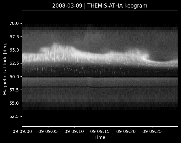
In making the last three plots, the geographic latitudes correspond to pixels mapped to a specified auroral emission altitude. This altitude is set with the alt kwarg passed into the ASI Interface Function. The default altitude is 110 km for THEMIS and 230 km for REGO.
If you pick an incorrect alt, you will get an error.
[13]:
try:
    asilib.asi.themis(location_code, time_range=time_range, alt=100)
except AssertionError as err:
    print('AssetionError:', err)
AssetionError: 100 km is not in the valid skymap altitudes: [ 90. 110. 150.] km. If you want a custom altitude with less percision, please use the custom_alt keyword
These auroral emission altitudes are defined in the skymap files.
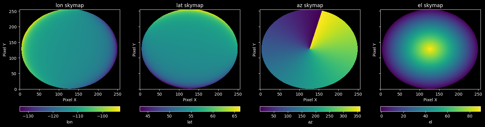
Skymap calibration files
You may wonder how the image’s pixel values were mapped to geographic latitude. This is done via the skymap calibration files that are provided by the instrument teams. They contain four arrays that map the ASI’s pixels to:
el- elevationaz- azimuthlat- latitudelon- longitude
These skymaps are essential for mapping images onto a geographic map, and for calculating the auroral intensity for conjunction studies.
[14]:
asi2.skymap.keys()
[14]:
dict_keys(['lat', 'lon', 'alt', 'el', 'az', 'path'])
What do these arrays look like?
[18]:
fig, ax = plt.subplots(1, 4, figsize=(20, 5), sharex=True, sharey=True)

for ax_i, key in zip(ax, ['lon', 'lat', 'az', 'el']):
    im = ax_i.imshow(asi2.skymap[key], origin='lower', aspect='auto')
    plt.colorbar(im, ax=ax_i, label=key, orientation='horizontal')
    ax_i.set_title(key+' skymap')
    ax_i.set_xlabel('Pixel X')
    ax_i.set_ylabel('Pixel Y')
The ASI maintainers often move or adjust their ASIs, after which a new skymap is often produced. Therefore, the relevant skymap is the one taken right before the images that were loaded. By default, asilib downloads all of the skymaps. The skymap file name below indicates that it is valid for images taken between 1 March 2007 and 22 May 2009.
[15]:
asi2.skymap['path'].name
[15]:
'themis_skymap_atha_20070301-20090522_vXX.sav'
Lastly, the Imager instance has a meta attribute that contains the ASI metadata such as location, pixel resolution, and cadence.
[16]:
asi2.meta
[16]:
{'array': 'THEMIS',
 'location': 'ATHA',
 'lat': 54.720001220703125,
 'lon': -113.30999755859375,
 'alt': 0.676,
 'cadence': 3,
 'resolution': (256, 256)}
You can also see human-readable summary of the ASI by printing it.
[17]:
print(asi2)
A THEMIS-ATHA Imager. time_range=[datetime.datetime(2008, 3, 9, 9, 0), datetime.datetime(2008, 3, 9, 9, 30)]
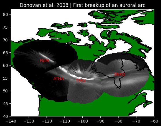
Mapping multiple all-sky images
You can plot one image from multiple ASI locations using a for-loop. In the following example, we will replicate Fig. 2b from:
Donovan, E., Liu, W., Liang, J., Spanswick, E., Voronkov, I., Connors, M., … & Rae, I. J. (2008). Simultaneous THEMIS in situ and auroral observations of a small substorm. Geophysical Research Letters, 35(17).
[18]:
time = datetime(2007, 3, 13, 5, 8, 45)
location_codes = ['FSIM', 'ATHA', 'TPAS', 'SNKQ']
map_alt = 110
min_elevation = 2  # Plot only pixels observed above some minimum elevation.

bx = asilib.map.create_simple_map()

asis = asilib.Imagers(
    [asilib.asi.themis(location_code, time=time, alt=map_alt) for location_code in location_codes]
    )
asis.plot_map(ax=bx, min_elevation=min_elevation)

bx.set_title('Donovan et al. 2008 | First breakup of an auroral arc')
plt.show()
/home/msshumko/research/.venv/lib/python3.14/site-packages/scipy/io/_idl.py:249: UserWarning: Not able to verify number of bytes from header
  structure[col['name']][i] = _read_structure(f,
/home/msshumko/research/.venv/lib/python3.14/site-packages/scipy/io/_idl.py:354: UserWarning: Not able to verify number of bytes from header
  record['data'] = _read_structure(f, rectypedesc['array_desc'],
Working with multiple images
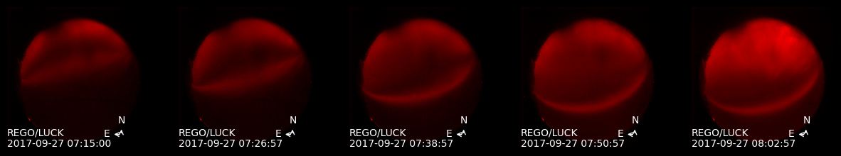
asilib.Imager supports slicing by time. In the example below, we plot a few fisheye and mapped images of STEVE that was observed by the REGO imagers.
Gallardo-Lacourt, B., Nishimura, Y., Donovan, E., Gillies, D. M., Perry, G. W., Archer, W. E., et al. (2018). A statistical analysis of STEVE. Journal of Geophysical Research: Space Physics, 123, 9893– 9905. https://doi.org/10.1029/2018JA025368
[19]:
time_range = [datetime(2017, 9, 27, 7, 15), datetime(2017, 9, 27, 8, 15)]
n_plots = 5
dt = int((time_range[1]-time_range[0]).total_seconds()/n_plots)
image_times = [time_range[0]+timedelta(seconds=i*dt) for i in range(n_plots)]

asi = asilib.asi.rego('LUCK', time_range=time_range)

fig, cx = plt.subplots(1, n_plots, figsize=(15, 8))

for montage_time, cx_i in zip(image_times, cx):
    filtered_asi = asi[montage_time]
    filtered_asi.plot_fisheye(ax=cx_i)
    cx_i.axis('off')
Redline Emission Geospace Observatory (REGO) data is courtesy of Space Environment Canada (space-environment.ca). Use of the data must adhere to the rules of the road for that dataset. Please see below for the required data acknowledgement. Any questions about the REGO instrumentation or data should be directed to the University of Calgary, Emma Spanswick (elspansw@ucalgary.ca) and/or Eric Donovan (edonovan@ucalgary.ca).

"The Redline Emission Geospace Observatory (REGO) is a joint Canada Foundation for Innovation and Canadian Space Agency project developed by the University of Calgary. REGO is operated and maintained by Space Environment Canada with the support of the Canadian Space Agency (CSA) [23SUGOSEC]."
Animate images
Let’s now make a simple fisheye lens movie of a substorm using Imager.animate_fisheye().
[20]:
location_code = 'FSMI'
time_range = [datetime(2015, 3, 26, 6, 7, 0), datetime(2015, 3, 26, 6, 30, 0)]

# loglevel is to suppress the verbose ffmpeg output.
asi = asilib.asi.themis(location_code, time_range=time_range)
asi.animate_fisheye(overwrite=True, ffmpeg_params={'loglevel':'quiet'})
plt.close()  # To show a clean output in this tutorial---it is often unnecessary.

# When you run this, you should see the video below in your asilib-data/movies directory.
Video('https://github.com/mshumko/asilib/raw/main/docs/_static/example_outputs/20150326_060700_063000_themis_fsmi_fisheye.mp4')
20150326_060700_063000_themis_fsmi_fisheye.mp4: |#######################| 100%
Animation saved to /mnt/f/asilib-data/animations/20150326_060700_063000_themis_fsmi_fisheye.mp4
[20]:
Animating images projected onto a map is also straightforward.
[21]:
location_code = 'FSMI'
time_range = [datetime(2015, 3, 26, 6, 7, 0), datetime(2015, 3, 26, 6, 30, 0)]

# loglevel is to suppress the verbose ffmpeg output.
asi = asilib.asi.themis(location_code, time_range=time_range)

lat_bounds = (asi.meta['lat']-7, asi.meta['lat']+7)
lon_bounds = (asi.meta['lon']-10, asi.meta['lon']+10)

dx = asilib.map.create_simple_map(lon_bounds=lon_bounds, lat_bounds=lat_bounds)
plt.subplots_adjust(top=0.99, bottom=0.05, left=0.05, right=0.99)

asi.animate_map(overwrite=True, ax=dx, ffmpeg_params={'loglevel':'quiet'})

plt.close()  # To show a clean output in this tutorial---it is often unnecessary.

# When you run this, you should see the video below in your asilib-data/animations directory.
Video('https://github.com/mshumko/asilib/raw/main/docs/_static/example_outputs/20150326_060700_061200_themis_fsmi_map.mp4')
20150326_060700_063000_themis_fsmi_map.mp4: |###########################| 100%
Animation saved to /mnt/f/asilib-data/animations/20150326_060700_063000_themis_fsmi_map.mp4
[21]:
If you need to annotate the animation, asilib.Imager has animate_fisheye_gen and animate_map_gen generator functions. After it plots each auroral image, it allows you to superpose your data.
Note: in each iteration, these methods do not clear the subplot; all plot objects persist unless you explicitly remove them
[22]:
location_code = 'FSMI'
time_range = [datetime(2015, 3, 26, 6, 10, 0), datetime(2015, 3, 26, 6, 30, 0)]

# loglevel is to suppress the verbose ffmpeg output.
asi = asilib.asi.themis(location_code, time_range=time_range)

lat_bounds = (asi.meta['lat']-7, asi.meta['lat']+7)
lon_bounds = (asi.  meta['lon']-10, asi.meta['lon']+10)

ex = asilib.map.create_simple_map(lon_bounds=lon_bounds, lat_bounds=lat_bounds)
plt.subplots_adjust(top=0.99, bottom=0.05, left=0.05, right=0.99)
gen = asi.animate_map_gen(overwrite=True, ax=ex, ffmpeg_params={'loglevel':'quiet'}, asi_label=False)

for time, image, ax, im in gen:
    if 'time_label' in locals():
        # This is one way I found to clean up an added plotting object.
        time_label.remove()
    time_label = ex.text(0.99, 0.99, f'location: {location_code} | time: {time}',
                         ha='right', va='top', transform=ex.transAxes, fontsize=15)

plt.close()  # To show a clean output in this tutorial---it is often unnecessary.

# When you run this, you should see the video below in your asilib-data/animations directory.
Video('https://github.com/mshumko/asilib/raw/main/docs/_static/example_outputs/20150326_061000_063000_themis_fsmi_map.mp4')
20150326_061000_063000_themis_fsmi_map.mp4: |###########################| 100%
Animation saved to /mnt/f/asilib-data/animations/20150326_061000_063000_themis_fsmi_map.mp4
[22]: