Examples
This example gallery using the best practices and illustrates functionality throughout asilib. These are complete examples that are also included in the asilib/examples/ directory on GitHub.
Fisheye Lens View of an Arc
A bright auroral arc that was analyzed by Imajo et al. 2021 “Active auroral arc powered by accelerated electrons from very high altitudes”

from datetime import datetime

import matplotlib.pyplot as plt

import asilib.asi

location_code = 'RANK'
time = datetime(2017, 9, 15, 2, 34, 0)

asi = asilib.asi.themis(location_code, time=time)
ax, im = asi.plot_fisheye()
plt.colorbar(im)
ax.axis('off')
plt.show()
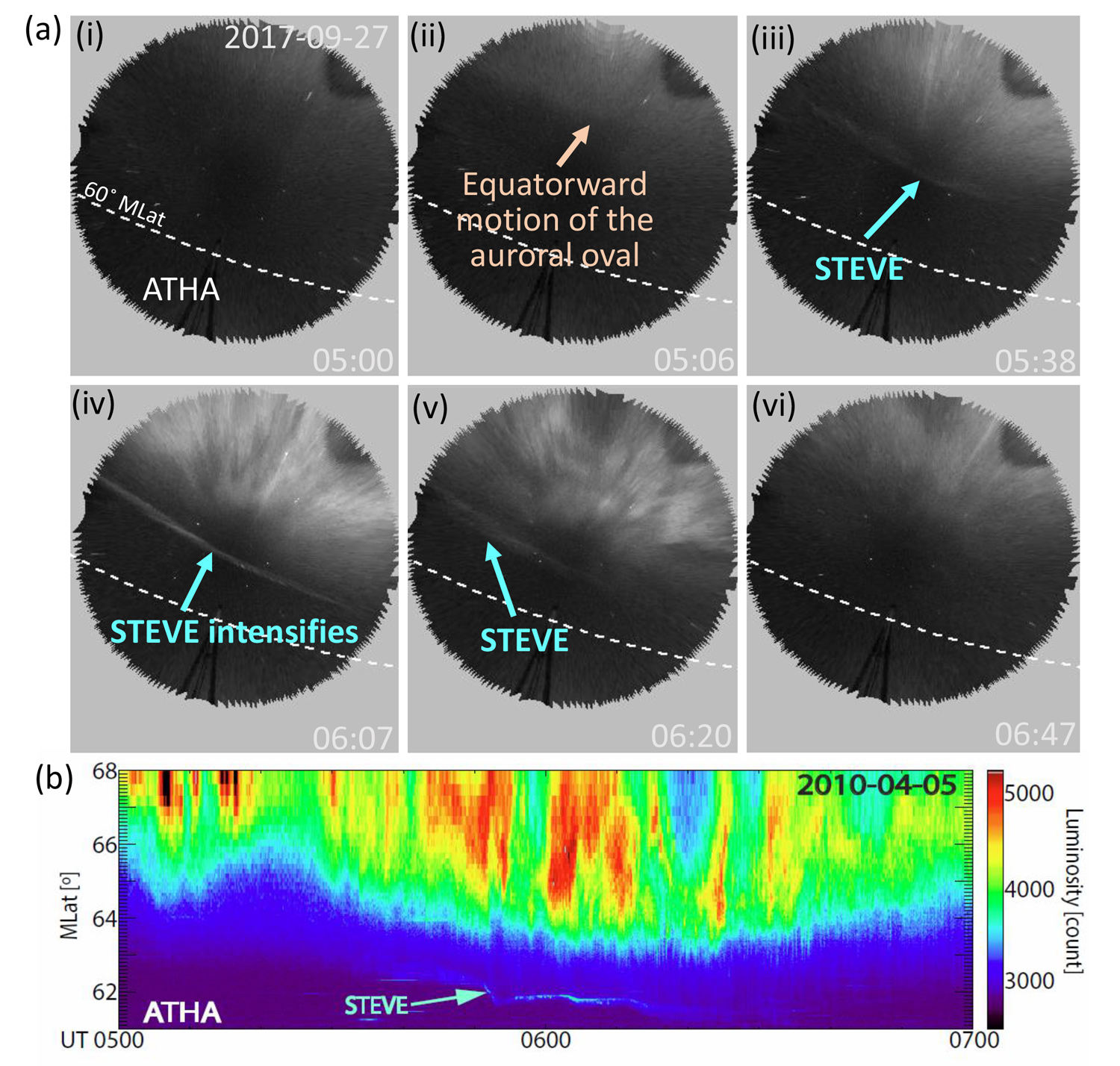
STEVE projected onto a map
Maps an image of STEVE (the thin band). Reproduced from http://themis.igpp.ucla.edu/nuggets/nuggets_2018/Gallardo-Lacourt/fig2.jpg

from datetime import datetime

import matplotlib.pyplot as plt

import asilib.asi
import asilib.map

ax = asilib.map.create_map(lon_bounds=(-127, -100), lat_bounds=(45, 65))

asi = asilib.asi.themis('ATHA', time=datetime(2010, 4, 5, 6, 7, 0), alt=110)
asi.plot_map(ax=ax)
plt.tight_layout()
plt.show()
Auroral arc projected onto a map
The first breakup of an auroral arc during a substorm analyzed by Donovan et al. 2008 “Simultaneous THEMIS in situ and auroral observations of a small substorm”

from datetime import datetime

import matplotlib.pyplot as plt

import asilib
import asilib.map
import asilib.asi

time = datetime(2007, 3, 13, 5, 8, 45)
location_codes = ['FSIM', 'ATHA', 'TPAS', 'SNKQ']
map_alt = 110
min_elevation = 2

ax = asilib.map.create_simple_map(lon_bounds=(-140, -60), lat_bounds=(40, 82))

_imagers = []

for location_code in location_codes:
    _imagers.append(asilib.asi.themis(location_code, time=time, alt=map_alt))

asis = asilib.Imagers(_imagers)
asis.plot_map(ax=ax, overlap=False, min_elevation=min_elevation)

ax.set_title('Donovan et al. 2008 | First breakup of an auroral arc')
plt.show()
Find Overlapping Pixels in a Mosaic
import asilib.asi
import asilib.map
import matplotlib.pyplot as plt
import cartopy.crs as ccrs

time = datetime(2007, 3, 13, 5, 8, 45)
location_codes = ['ATHA', 'TPAS']
map_alt = 110
_imagers = [asilib.asi.themis(location_code, time=time, alt=map_alt)
            for location_code in location_codes]
asis = asilib.Imagers(_imagers)
overlapping_masks = asis.find_overlap_pixels(min_elevation=2)

ax = asilib.map.create_map(
    lon_bounds=(-125, -90), lat_bounds=(42, 64)
    )

asis.plot_map(ax=ax, min_elevation=2)

asi_names = [f'{_imager.meta["array"]}-{_imager.meta["location"]}' for _imager in asis.imagers]

for self_loc, neighbors in overlapping_masks.items():
    for neighbor_loc, overlapping_mask in neighbors.items():
        self_loc_idx = asi_names.index(self_loc)
        neighbor_loc_idx = asi_names.index(neighbor_loc)
        ax.scatter(
            asis.imagers[self_loc_idx].skymap['lon'][overlapping_mask],
            asis.imagers[self_loc_idx].skymap['lat'][overlapping_mask],
            alpha=0.5,
            label=f'{self_loc} pixels overlapping with {neighbor_loc}',
            s=2,
            transform=ccrs.PlateCarree()
        )

ax.legend(loc='lower left', fontsize=12, markerscale=3)
plt.tight_layout()
plt.show()
A keogram of STEVE
A keogram with a STEVE event that moved towards the equator. This event was analyzed in Gallardo-Lacourt et al. 2018 “A statistical analysis of STEVE”

import matplotlib.pyplot as plt

import asilib.asi

location_code = 'LUCK'
time_range = ['2017-09-27T07', '2017-09-27T09']
map_alt_km = 230

fig, ax = plt.subplots(figsize=(8, 6))
asi = asilib.asi.rego(location_code, time_range=time_range, alt=map_alt_km)
ax, p = asi.plot_keogram(ax=ax, color_bounds=(300, 800), aacgm=True)
plt.colorbar(p, label='Intensity')
ax.set_xlabel('UTC')
ax.set_ylabel(f'Magnetic Latitude [deg]\nEmission altitude={map_alt_km} km')
plt.tight_layout()
plt.show()
Keogram of a field line resonance
A field line resonance studied in: Gillies, D. M., Knudsen, D., Rankin, R., Milan, S., & Donovan, E. (2018). A statistical survey of the 630.0-nm optical signature of periodic auroral arcs resulting from magnetospheric field line resonances. Geophysical Research Letters, 45(10), 4648-4655.

import matplotlib.pyplot as plt

import asilib.asi

location_code = 'GILL'
time_range = ['2015-02-02T10', '2015-02-02T11']

asi = asilib.asi.rego(location_code, time_range=time_range, alt=230)
ax, p = asi.plot_keogram(color_map='Greys_r')
plt.xlabel('Time')
plt.ylabel('Geographic Latitude [deg]')
plt.colorbar(p)
plt.tight_layout()
plt.show()
Fisheye Movie
from datetime import datetime

import asilib.asi

location_code = 'FSMI'
time_range = (datetime(2015, 3, 26, 6, 7), datetime(2015, 3, 26, 6, 30))
asi = asilib.asi.themis(location_code, time_range=time_range)
asi.animate_fisheye()

print(f'Animation saved in {asilib.config["ASI_DATA_DIR"] / "animations" / asi.animation_name}')
Map movie
from datetime import datetime

import asilib.asi
import asilib.map

time_range = (datetime(2015, 3, 26, 6, 7), datetime(2015, 3, 26, 6, 12))
location_code = 'FSMI'

asi = asilib.asi.themis(location_code, time_range=time_range, alt=110)

lat_bounds = (asi.meta['lat'] - 7, asi.meta['lat'] + 7)
lon_bounds = (asi.meta['lon'] - 20, asi.meta['lon'] + 20)
ax = asilib.map.create_map(lon_bounds=lon_bounds, lat_bounds=lat_bounds)

asi.animate_map(ax=ax)

print(f'Animation saved in {asilib.config["ASI_DATA_DIR"] / "animations" / asi.animation_name}')
Animate Mosaic
import asilib
import asilib.asi

time_range = ('2021-11-04T06:55', '2021-11-04T07:05')
asis = asilib.Imagers(
    [asilib.asi.trex_rgb(location_code, time_range=time_range)
    for location_code in ['LUCK', 'PINA', 'GILL', 'RABB']]
    )
asis.animate_map(lon_bounds=(-115, -85), lat_bounds=(43, 63), overwrite=True)
ASI-satellite conjunction movie
A comprehensive example that maps a hypothetical satellite track to an image and calculates the mean ASI intensity in a 20x20 km box around the satellite’s 100 km altitude footprint.
from datetime import datetime

import numpy as np
import matplotlib.pyplot as plt

import asilib
import asilib.asi


# ASI parameters
location_code = 'RANK'
alt=110  # km
time_range = (datetime(2017, 9, 15, 2, 32, 0), datetime(2017, 9, 15, 2, 35, 0))

fig, ax = plt.subplots(
    3, 1, figsize=(7, 10), gridspec_kw={'height_ratios': [4, 1, 1]}, constrained_layout=True
)

asi = asilib.asi.themis(location_code, time_range=time_range, alt=alt)

# Create the fake satellite track coordinates: latitude, longitude, altitude (LLA).
# This is a north-south satellite track oriented to the east of the THEMIS/RANK
# imager.
n = int((time_range[1] - time_range[0]).total_seconds() / 3)  # 3 second cadence.
lats = np.linspace(asi.meta["lat"] + 5, asi.meta["lat"] - 5, n)
lons = (asi.meta["lon"] - 0.5) * np.ones(n)
alts = alt * np.ones(n)  # Altitude needs to be the same as the skymap.
sat_lla = np.array([lats, lons, alts]).T
# Normally the satellite time stamps are not the same as the ASI.
# You may need to call Conjunction.interp_sat() to find the LLA coordinates
# at the ASI timestamps.
sat_time = asi.data.time

conjunction_obj = asilib.Conjunction(asi, (sat_time, sat_lla))

# Map the satellite track to the imager's azimuth and elevation coordinates and
# image pixels. NOTE: the mapping is not along the magnetic field lines! You need
# to install IRBEM and then use conjunction.lla_footprint() before
# calling conjunction_obj.map_azel.
sat_azel, sat_azel_pixels = conjunction_obj.map_azel()

# Calculate the auroral intensity near the satellite and mean intensity within a 10x10 km area.
nearest_pixel_intensity = conjunction_obj.intensity(box=None)
area_intensity = conjunction_obj.intensity(box=(10, 10))
area_mask = conjunction_obj.equal_area(box=(10,10))

# Need to change masked NaNs to 0s so we can plot the rectangular area contours.
area_mask[np.where(np.isnan(area_mask))] = 0

# Initiate the animation generator function.
gen = asi.animate_fisheye_gen(
    ax=ax[0], azel_contours=True, overwrite=True, cardinal_directions='NE'
)

for i, (time, image, _, im) in enumerate(gen):
    # Plot the entire satellite track, its current location, and a 20x20 km box
    # around its location.
    ax[0].plot(sat_azel_pixels[:, 0], sat_azel_pixels[:, 1], 'red')
    ax[0].scatter(sat_azel_pixels[i, 0], sat_azel_pixels[i, 1], c='red', marker='o', s=50)
    ax[0].contour(area_mask[i, :, :], levels=[0.99], colors=['yellow'])

    if 'vline1' in locals():
        vline1.remove()  # noqa: F821
        vline2.remove()  # noqa: F821
        text_obj.remove()  # noqa: F821
    else:
        # Plot the ASI intensity along the satellite path
        ax[1].plot(sat_time, nearest_pixel_intensity)
        ax[2].plot(sat_time, area_intensity)
    vline1 = ax[1].axvline(time, c='b')
    vline2 = ax[2].axvline(time, c='b')

    # Annotate the location_code and satellite info in the top-left corner.
    location_code_str = (
        f'THEMIS/{location_code} '
        f'LLA=({asi.meta["lat"]:.2f}, '
        f'{asi.meta["lon"]:.2f}, {asi.meta["alt"]:.2f})'
    )
    satellite_str = f'Satellite LLA=({sat_lla[i, 0]:.2f}, {sat_lla[i, 1]:.2f}, {sat_lla[i, 2]:.2f})'
    text_obj = ax[0].text(
        0,
        1,
        location_code_str + '\n' + satellite_str,
        va='top',
        transform=ax[0].transAxes,
        color='red',
    )
    ax[1].set(ylabel='ASI intensity\nnearest pixel [counts]')
    ax[2].set(xlabel='Time', ylabel='ASI intensity\n10x10 km area [counts]')

print(f'Animation saved in {asilib.config["ASI_DATA_DIR"] / "animations" / asi.animation_name}')